Chapter 15 Extensions
15.1 Review
In this class, we’ve talked about how we can use concepts, models, measurements, and comparisons to carefully observe the political world.
We spent a little time talking about concepts, models, and measurements.
We spend most of the time talking about comparisons.
We talked about percentages, proportions, averages, and standard deviations. We noted that we might compare these across groups. For example, we compared the average ideology score for Republicans across Congresses (they’ve been shifting to the right.) We compared the turnout rate among those who received the “self mailer” to the rate for those that received the “neighbors mailer” (threatening to expose non-voters to their neighbors causes them to vote).
We talked about using correlation and regression to make comparisons directly. We examined Gamson’s Law (seat shares vary almost one-to-one with portfolio shares) and we examined the relationship between district magnitude and the effective number of parties (as magnitude goes up, so does the number of parties).
We noted that there are four ways to get a relationship between two variables:
- Causation
- Spuriousness
- Reverse Causation
- Chance
We talked about how we can use randomization (i.e., experiments) to eliminate the possibility that a correlation is due to spuriousness or reverse causation.
I mentioned that we would deal with chance later in the semester.
15.2 Sources of Randomness
At this point, we’ve used sample surveys to better understand how to deal with chance using confidence intervals and/or p-values.
In our application, chance always entered the data through random sampling.
In general, randomness enters our comparisons when we have any of the following:
- random sampling: the result differs from study to study because we get a different sample in each study.
- randomization: the result differs from study to study because we put different subjects in the treatment and control groups across the studies.
- imagining a stochastic world: if we rewound time and let the world play forward again, then idiosyncratic or “random” events would lead to different outcomes. The world we observe is just one of many possibilities. The observed world is like a random sample from the possible worlds.
The last—a stochastic world—seems a bit weird. In almost all cases, political scientists assume that the data the real world gives us (e.g., the nominate data, the parties dataset) have a random component. They imagine, at least in practice, that we can think of some parts of the outcome as “systematic” or “explainable” and other parts as “idiosyncratic”, “random,” or “unexplainable.” For example, suppose that you get a flat tire on Election Day and can’t make it to the polling place. We might think of that as a random event (like a coin toss) that stopped you from voting. Thus, whether or not you voted is partly systematic (your education, political interest, etc.) and partly random (e.g., flat tire, medical emergency, etc.). Unlike random sampling or randomization, this source of randomness is totally imaginary. But if we imagine it, we can model it.
15.3 Confidence Intervals in General
We focused our detailed applications narrowly on simple random samples and proportions.
But instead of proportions, we could have focused on averages, SDs, correlations, or regression slopes. Instead of simple random samples, we could have focused on randomization or imagined randomness.
The math would have been harder, but the logic is the same.
Because of the randomness, the dataset you have helps you estimate the quantity you really care about, but with some error. We can use confidence intervals to determine how close the estimate is to the quantity we care about.
Statisticians have developed many quantities to summarize a dataset and methods to estimate the SE for those quantities. Regardless of the quantity, the logic is always:
95% confidence interval = estimate +/- 2 SEs
(There are other ways to create a confidence interval, but this approach is common.)
The quantity we’re talking about might change from proportion to an average to a correlation to a slope to something you haven’t learned yet. The formula for the SE will change across these quantities. But the interpretation of the SE is always the same–the SE is the long run SD of the estimate if you repeat the study again-and-again.
15.4 Hypothesis Tests in General
As with confidence intervals, our discussion of hypothesis tests focused narrowly on simple random samples and proportions. Also like confidence intervals, that logic generalizes.
For a given null hypothesis about a particular quantity, statisticians have developed a method to compute the p-value. Regardless of the null hypothesis and regardless of the quantity of interest, the p-value is the probability that we would observe data at least as extreme as the observed data if the null hypothesis is true. If the p-value is less than or equal to 0.05, we reject the null hypothesis and accept the alternative. If the p-value is greater than 0.05, we acknowledge that the data are consistent with both the null and alternative hypotheses.
15.5 Statistical Significance
When we’re comparing averages or examining a regression slope, it’s common for political scientists to use “no difference” or “no relationship” as the null hypothesis. It’s so common, in fact, that political scientists rarely explicitly state the null hypothesis. When it’s not stated, you can assume that the researcher is using the hypotheses below.
- When comparing groups with a proportion, percent, or average:
- null hypothesis: no difference
- alternative hypothesis: any difference (positive or negative)
- When comparing variables with a correlation or a variable:
- null hypothesis: no relationship
- alternative hypothesis: any relationship (positive or negative)
When we reject the null hypothesis of no difference or relationship, we refer to the estimate as “statistically significant.” I don’t care for the term at all because “significant” seems to imply “important.” However, “statistically significant” is neither necessary nor sufficient for a statistical result to be important.
Say that an estimate of a difference or a relationship is statistically significant if you can reject the null hypothesis of no difference or no relationship.
In other words, when an estimate of a difference or relationship is statistically significant, you can confidently claim that the observed difference or relationship is not due to chance. It’s quite common to flag statistically significant estimates with stars. When you see an estimate flagged with a star, you know that it’s statistically significant.
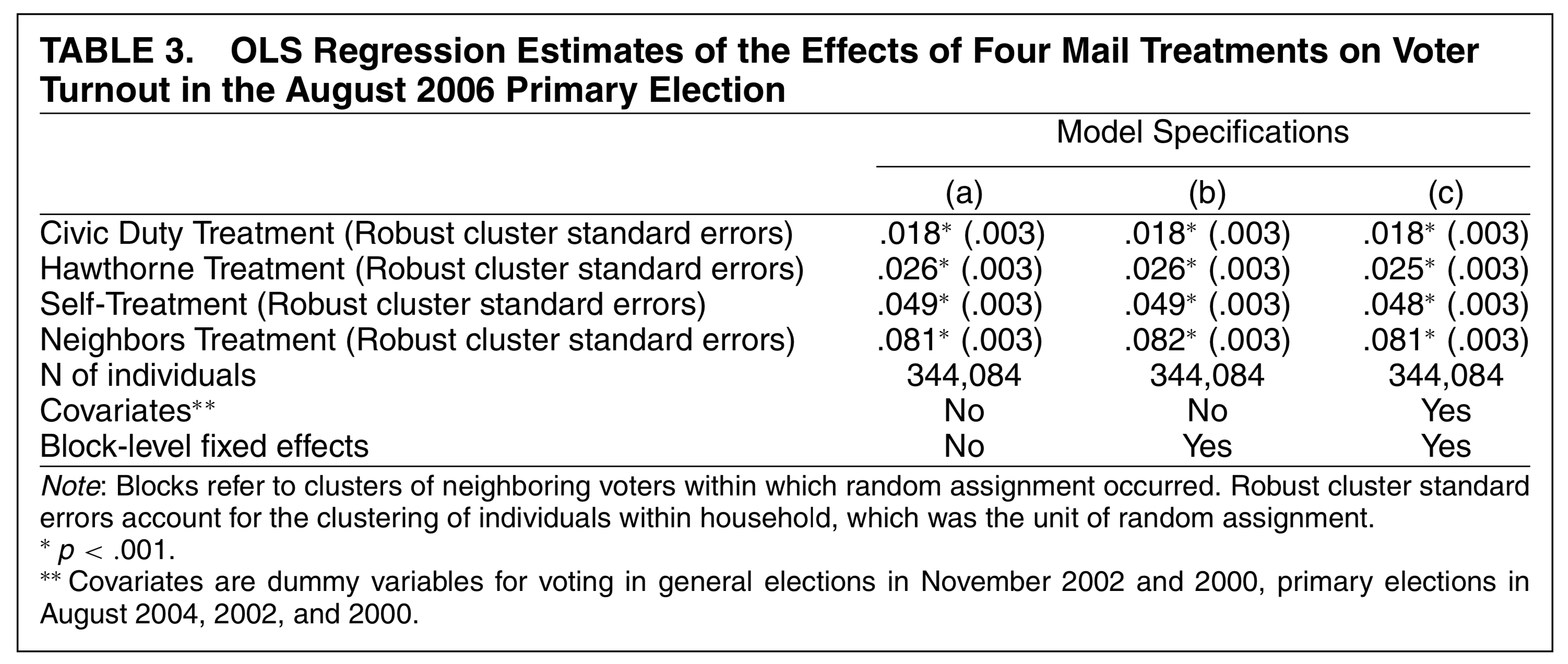
As an example, see Table 3 below from Gerber, Green, and Larimer (2008). The numbers are estimates of the treatment effect of each mailer (compared to the control group that received no mailer). Each estimate is statistically significant, which means we’re confident the observed differences are not due to chance.