Chapter 17 Fitting a Linear Regression Model in R

In these notes, we are going to re-analyze the data presented in Figure 12.4 from the Clark, Golder, and Golder (2013, pp. 477-478) reading. The necessary variables are in the data set gamson.rds. The data frame gamson has two variables: seat_share and portfolio_share.

# load packages
library(tidyverse)

# load data
gamson <- readRDS("gamson.rds")

# quick look at data
glimpse(gamson)

Rows: 826
Columns: 2
$ seat_share      <dbl> 0.02424242, 0.46060607, 0.51515150, 0.47204968, 0.5279…
$ portfolio_share <dbl> 0.09090909, 0.36363637, 0.54545456, 0.45454547, 0.5454…

This is a particularly useful data set on which to estimate a linear regression model. Remember that Gamson’s Law states that “cabinet portfolios will be distributed among government parties in strict proportion to the number of seats that each party contributes to the government’s legislative majority.”

Gamson’s Law implies that legislative seat shares should (according to the Law) relate to government portfolios linearly, with an intercept of zero and a slope of one. The slope should equal one because a one percentage point increase in seat share ought to lead to a one percentage point increase in portfolio share, at least on average. The intercept should equal zero because we expect a party with 0% of the legislative seats to get 0% of the government portfolios.

To fit a linear regression model, we use the lm() function. (The “l” stands for “linear” and the “m” stands for “model.”)

The lm() function takes two arguments:

• The first argument to lm() is called a formula. For simple linear models with only one predictor, the formula has the form y ~ x, where y is the outcome (or “dependent variable”) and x is the explanatory variable (or “independent variable” or “predictor”). I usually put the formula first and leave the argument implicit.
• The second argument to lm() is the data argument. This will be the data frame in which to find x and y. I usually put this argument second and make it explicit.

In the case of the data frame gamson, our y is portfolio_share, our x is seat_share, and our data is gamson.

# fit linear model
fit <- lm(portfolio_share ~ seat_share, data = gamson)

Now we have used the lm() function to fit the model and stored the output in the object fit. So what type of object is fit? It turns out that lm() outputs a new type of object called a “list” that is like a vector, but more general. Whereas we think of a vector as collections of numbers (or character strings, etc.), we can think of lists as collection of R objects. The collection objects in the list can be scalars, functions, vectors, data frames, or other lists. This turns out to not be practically important to us, since we will not work directly with lists in this class.

Instead of working directly with fit, which is a list, we’ll use other functions to compute quantities that interest us.

17.1 Model Coefficients

First, we might care about the coefficients. In the case of a model with only one explanatory variable, we’ll just have an intercept and a slope. The coef() function takes one argument–the output of the lm() function, which we stored as the object fit–and returns the estimated coefficients.

coef(fit)

(Intercept)  seat_share 
 0.06913558  0.79158398 

We can see that Gamson’s Law isn’t exactly correct, a one-unit percentage point increase in vote share least to about a 0.8 percentage point increase in the portfolio share. Also, the intercept is slightly above zero, suggesting that smaller parties have a disproportionate advantage.

17.2 R.M.S. Error

We might also be interested in the r.m.s. error of the model. The function residuals() works just like coef(), except it returns the model errors (i.e., “residuals”) instead of the model coefficients. Surprisingly, there is no function that automatically calculates the r.m.s. in R (without loading a package), so we’ll have to calculate it ourselves.

# one step at a time, r.m.s. error
e <- residuals(fit)
se <- e^2
mse <- mean(se)
rmse <- sqrt(mse)
print(rmse)  # r.m.s. error

[1] 0.06880963

# all at once
sqrt(mean(residuals(fit)^2))  # r.m.s. error

[1] 0.06880963

For now, all we are really interested in is the coefficients and the r.m.s. error, so these two are all we need.

We can coefficients and RMS error of the residuals using the display() function from the arm package. We can see the intercept is 0.07, the slope is 0.79, and the RMS of the residuals (or “residual sd”) is 0.07.

arm::display(fit)

lm(formula = portfolio_share ~ seat_share, data = gamson)
            coef.est coef.se
(Intercept) 0.07     0.00   
seat_share  0.79     0.01   
---
n = 826, k = 2
residual sd = 0.07, R-Squared = 0.89

17.3 Adding the Regression Line in ggplot

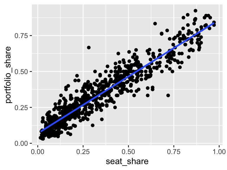
Whenever we draw a scatterplot, we’ll usually want to draw the regression line through the data. That is done by adding geom_smooth() to the plot. We’ll usually want to supply two arguments to geom_smooth(). First, we’ll want to set method = "lm" so that geom_smooth() fits a line through the data, as opposed to a smooth curve. Second, we’ll want to set se = FALSE so that geom_smooth() does not include the standard error, which we haven’t discussed yet (that’s the last third of the class).

# create scatterplot with regression line
ggplot(gamson, aes(x = seat_share, y = portfolio_share)) + 
  geom_point() + 
  geom_smooth(method = "lm", se = FALSE)